Day 4 – Introduction to Scikit-Learn: Building ML Models

Introduction

By 2025, Scikit-Learn has solidified its place as the gateway library for machine learning in Python. At CuriosityTech.in (Nagpur, Wardha Road, Gajanan Nagar), we guide learners to use Scikit-Learn as a hands-on laboratory for building, evaluating, and understanding ML models before they transition to deep learning or deployment.

Scikit-Learn is versatile, beginner-friendly, and widely adopted in industry. Whether you’re preparing for ML engineer interviews or real-world projects, understanding this library is mandatory.

This blog is structured like a Lab Manual, so you can follow it step by step, as if you were sitting in a real ML lab.

Lab Objective

Required Tools

• Python 3.9+

• Jupyter Notebook / VSCode

• Libraries: numpy, pandas, matplotlib, scikit-learn

Tip from CuriosityTech.in: Always work in virtual environments to avoid library conflicts.

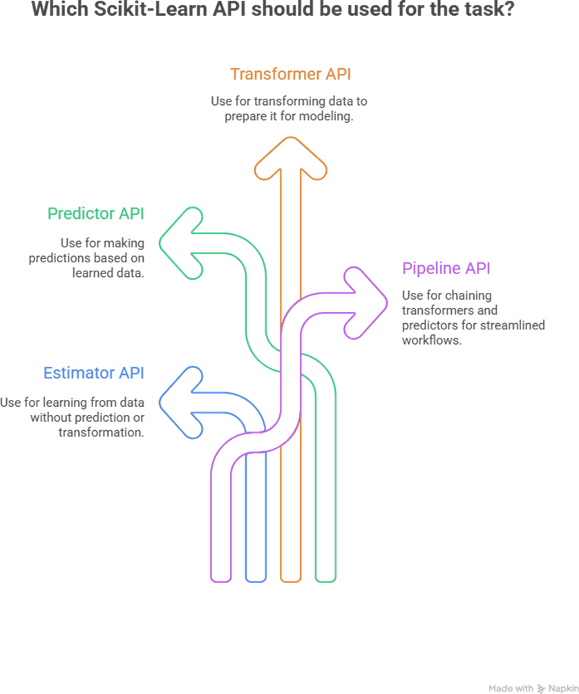
Step 1: Understanding Scikit-Learn Architecture

Step 2: Loading a Dataset

For beginners, Scikit-Learn provides sample datasets. We’ll use the classic Iris dataset for classification.

from sklearn.datasets import load_iris data = load_iris()

X = data.data y = data.target

• X → features (sepal length, petal width, etc.)

• y → target (species)

At CuriosityTech.in, our students practice on both sample datasets and real-world datasets (like CSVs from Kaggle) to bridge theory and industry applications.

Step 3: Splitting Data

To evaluate model performance, we split the dataset into training and testing sets.

from sklearn.model_selection import train_test_split

X_train, X_test, y_train, y_test = train_test_split(X, y, test_size=0.2, random_state=42)

Lab Tip:

• Use 70-80% for training and 20-30% for testing.

• Always set random_state for reproducibility.

Step 4: Building a Classification Model

Let’s build a Logistic Regression model.

from sklearn.linear_model import LogisticRegression model = LogisticRegression()

model.fit(X_train, y_train)

y_pred = model.predict(X_test)

• .fit() → Learns from training data

• .predict() → Makes predictions on unseen data

At Curiosity Tech Park, beginners often practice multiple models to compare which performs best.

Step 5: Model Evaluation

Accuracy is just one metric. Scikit-Learn provides:

• Accuracy, Precision, Recall, F1-score

• Confusion matrix for classification

from sklearn.metrics import accuracy_score, classification_report print(“Accuracy:”, accuracy_score(y_test, y_pred)) print(classification_report(y_test, y_pred))

Lab Observation: Understanding metrics helps you choose the right model for the business problem, not just the one with the highest accuracy.

Step 6: Regression Example

Let’s also build a Linear Regression model on a synthetic dataset:

from sklearn.datasets import make_regression

X, y = make_regression(n_samples=100, n_features=1, noise=10, random_state=42)

from sklearn.model_selection import train_test_split

X_train, X_test, y_train, y_test = train_test_split(X, y, test_size=0.2, random_state=42)

from sklearn.linear_model import LinearRegression reg_model = LinearRegression() reg_model.fit(X_train, y_train)

y_pred = reg_model.predict(X_test)

Visualization:

import matplotlib.pyplot as plt

plt.scatter(X_test, y_test, color=’blue’, label=’Actual’) plt.plot(X_test, y_pred, color=’red’, label=’Predicted’) plt.legend()

plt.show()

This gives a clear visual of model performance. CuriosityTech students often practice such regression labs to understand how model predictions align with reality.

Step 7: Using Pipelines for Workflow Automation

Instead of manually applying transformations and fitting models: from sklearn.preprocessing import StandardScaler from sklearn.pipeline import Pipeline

pipeline = Pipeline([

(‘scaler’, StandardScaler()), (‘log_reg’, LogisticRegression())

])

pipeline.fit(X_train, y_train) y_pred = pipeline.predict(X_test)

• Scalers standardize data

• Pipeline chains steps → cleaner, production-ready code

At CuriosityTech.in, we emphasize pipelines because real-world ML isn’t just about modeling—it’s about reproducibility and scalability.

Step 8: Experimenting Like a Pro

Lab Exercise Suggestions:

1. Compare Logistic Regression vs Random Forest for Iris dataset.

• Test different train-test splits and observe accuracy variance.

• Implement K-Fold Cross-Validation to evaluate model stability.

Pro Tip: Every exercise at CuriosityTech Nagpur is designed to simulate real industry challenges, preparing students for 2025 ML demands.

Infographic / Diagram (Description for Blog)

• Diagram showing ML Pipeline with Scikit-Learn:

• Raw Data → Preprocessing (Transformer) → Model Training (Estimator)

→ Prediction → Evaluation

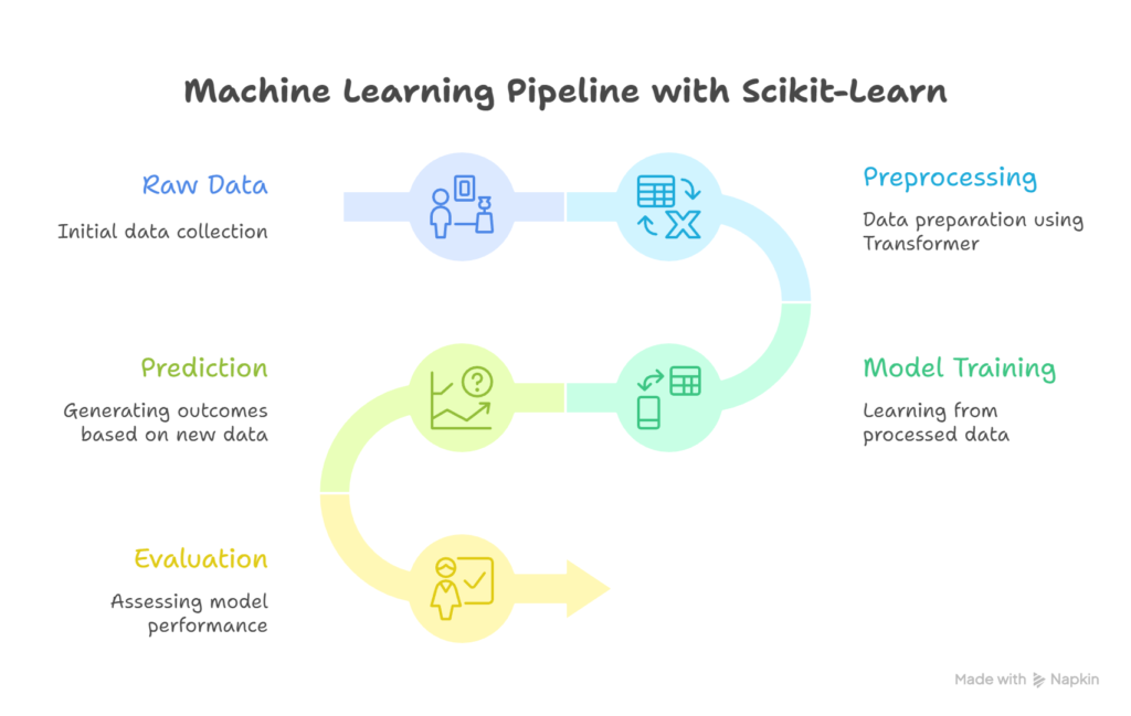
• Side annotation: “CuriosityTech mentors help you navigate each step with real-world examples.”

Step 9: Real-World Applications

• ​

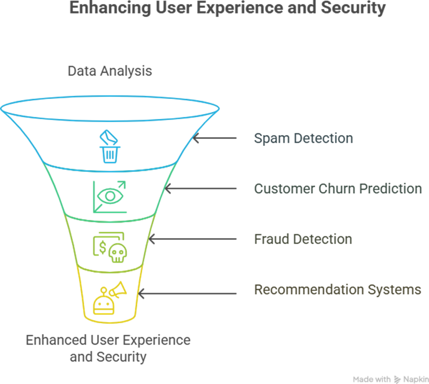
At CuriosityTech.in, students build these as mini-projects before progressing to deep learning or deployment workflows.

Step 10: Key Takeaways

1. Scikit-Learn simplifies model building with fit, predict, and transform methods.

• Pipelines make workflows efficient, reproducible, and production-ready.

• Evaluation metrics guide real decisions, not just theoretical learning.

• Hands-on practice is non-negotiable for expertise in ML.

As we often tell students: “Master the lab first, and the field will be easy to conquer.”

Conclusion

Scikit-Learn is the first bridge between learning ML theory and building practical solutions. By mastering this library, you can:

• Build regression and classification models

• Evaluate models effectively

• Automate ML workflows for production

At CuriosityTech Nagpur, every learner gets personal guidance, real-world case studies, and a roadmap from Scikit-Learn basics to full ML pipelines. Connecting with us via contact@curiositytech.in or +91-9860555369 ensures your ML journey is guided, hands-on, and industry-aligned.